Introduction
Predicting total wealth using various economic indicators has long intrigued economists. This paper aims to predict an individual’s total wealth through statistical learning methods, utilizing data from the 1991 Survey of Income and Program Participation (SIPP). The dataset comprises 7,933 observations, with the following variables used as predictors:
ira: Individual retirement account (IRA) in US dollarse401: Eligibility for 401(k) (1 if eligible, 0 otherwise)nifa: Non-401(k) financial assets in US dollarsinc: Income in US dollarshmort: Home mortgage in US dollarshval: Home value in US dollarshequity: Home equity (home value minus home mortgage)educ: Education in yearsmale: Gender (1 if male, 0 otherwise)twoearn: Dual-income households (1 if two earners, 0 otherwise)nohs,hs,smcol,col: Educational attainment dummiesage: Agefsize: Family sizemarr: Marital status (1 if married, 0 otherwise)
The sample includes households where the reference person is aged 25–64, at least one person is employed, and no one is self-employed. The observation units correspond to household reference persons.
Preliminary Analysis
Initial examination revealed perfect collinearity among home mortgage (hmort), home value (hval), and home equity (hequity), so hequity was excluded. The educational attainment dummies serve the same purpose as the educ variable and were also omitted.
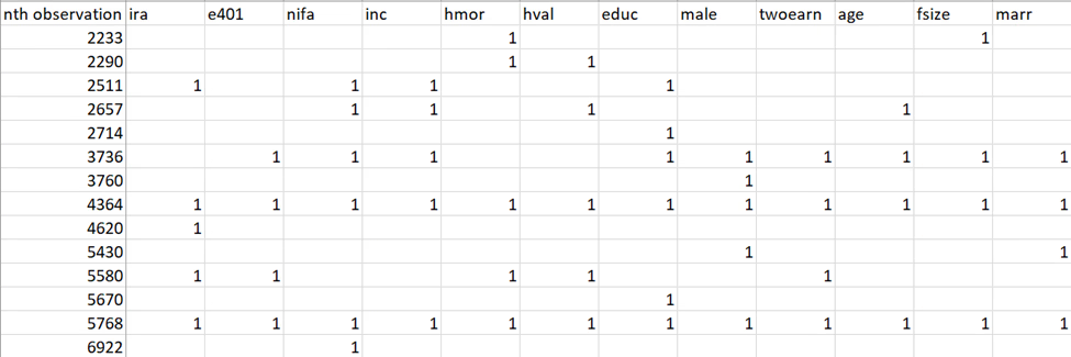
Before building models, outliers and high-leverage points needed to be removed since these observations have sizable impact on the estimated regression line. According to An Introduction to Statistical Learning, high leverage points are “cause for concern if the least squares line is heavily affected by just a couple of observations, because any problems with these points may invalidate the entire fit” (Gareth et al. 98). Outliers were identified through Residuals vs. Fitted plots, and high leverage points through Residuals vs. Leverage plots. After removing flagged observations, 7,919 observations remained.
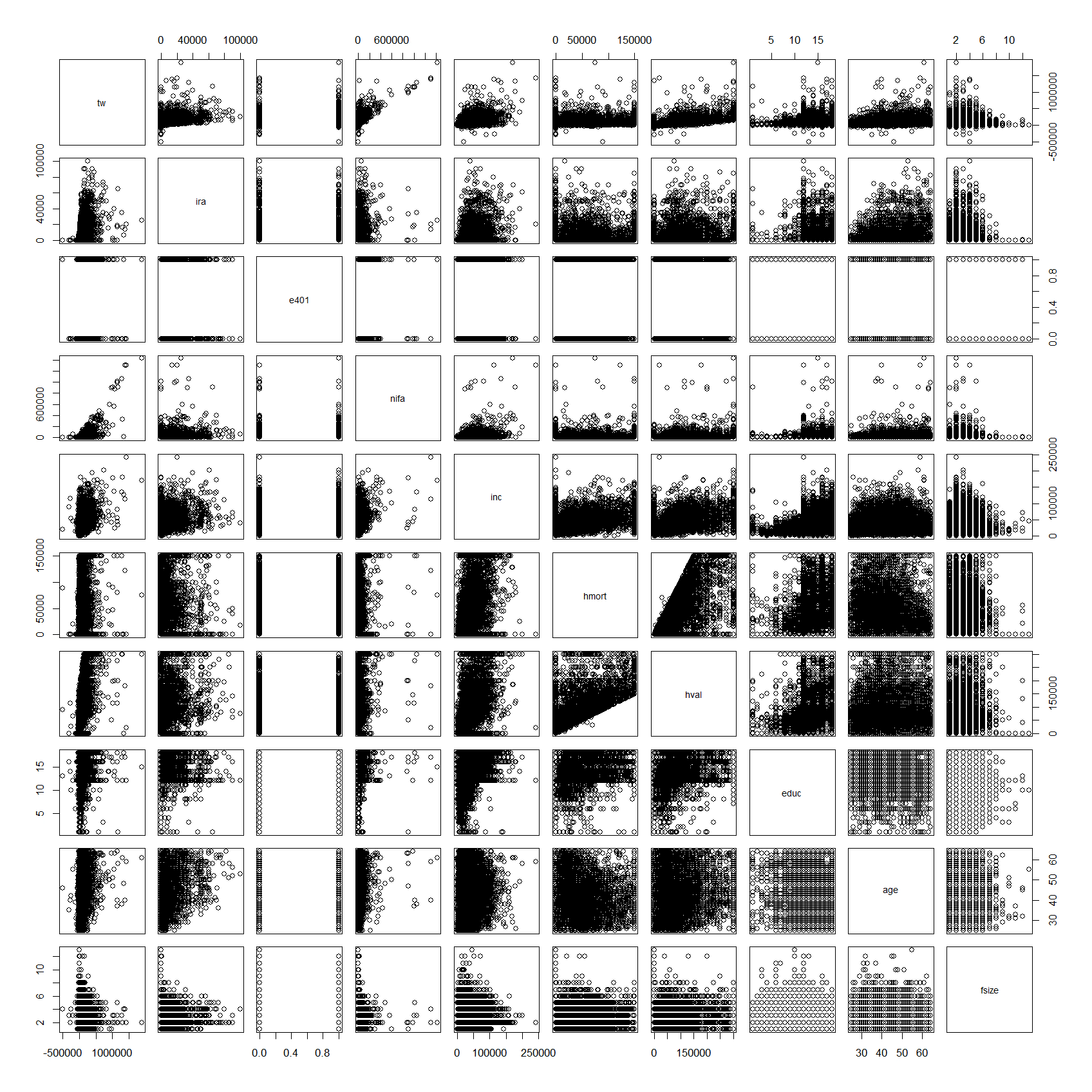
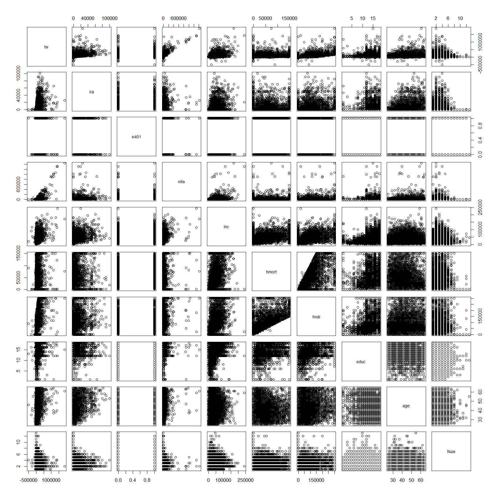
The scatterplot matrix indicated non-linear relationships between total wealth and ira, e401, nifa, inc, educ, age, and fsize.
Not all non-linearities were statistically significant. Backward stepwise selection identified the following as significant predictors: ira, e401, nifa, inc, hmort, hval, male, twoearn, and age.
Natural cubic splines were employed on ira, nifa, inc, and age. Natural cubic splines were chosen over cubic splines because they handle large datasets more effectively and avoid abrupt jumps in predictions. Ten-fold cross-validation determined optimal degrees of freedom of 11, 11, and 3 for ira, nifa, and age respectively. For inc, zero knots had the lowest MSPE, so no transformation was applied.
In-depth Analysis
Further analysis compared LASSO, Ridge, and Stepwise regressions, all assessed through ten-fold cross-validation. Backward stepwise regression performed best, with the lowest Mean Squared Prediction Error (MSPE): 1,365,955,376.
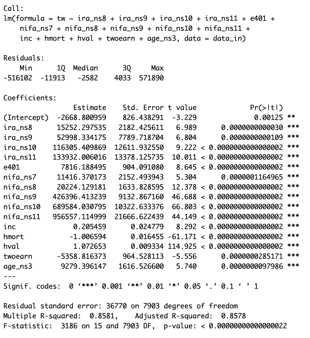
Since this MSPE was quite large, a Generalized Additive Model (GAM) was fitted using only the statistically significant variables from backward stepwise regression. The final model:
lm(formula = tw ~ ira_ns8 + ira_ns9 + ira_ns10 + e401 +
   nifa_ns7 + nifa_ns8 + nifa_ns9 + nifa_ns10 + nifa_ns11 +
   inc + hmort + hval + twoearn + age, data = data_in)
Results Summary
Residuals: The median prediction error is quite low, though there are large outliers. Given how household total wealth varies in reality, these are acceptable.
Coefficients: The spline term coefficients capture the non-linear relationships between ira, nifa, and total wealth. The high significance of these coefficients indicates that the spline transformations are effectively modeling complex relationships.
Model Performance: Adjusted R-squared of 0.858 indicates that approximately 85.8% of variance in total wealth is explained by the model. The high F-statistic and low p-value indicate the model is highly statistically significant.
Conclusion
The Generalized Additive Model provided the best fit among the models tested. Key findings:
- IRAs: Non-linear relationship suggests impact varies at different contribution levels.
- 401(k) eligibility: Indicates whether the household head is employed.
- Non-401(k) financial assets: Complex non-linear relationship with a slightly positive overall correlation.
- Income: Each additional dollar of income associated with $0.19 increase in total wealth, on average.
- Home value and mortgage: Each dollar increase in home value associated with $1.07 increase in wealth; each dollar of mortgage with $1.01 decrease. Home equity plays a significant role.
- Age: Each year associated with average increase of $250.85, reflecting asset accumulation.
- Two-earner households: Surprisingly associated with $4,751 less in total wealth than single-earner households, potentially due to factors not captured such as childcare costs.
Future research could explore additional variables or alternative modeling techniques to further refine predictions.
Citation
James, Gareth, et al. An Introduction to Statistical Learning: with Applications in R. Springer, 2017.
Metadata
- Duration: February 2021 – March 2021
- Responsibilities: Statistical analysis using R and writing